Learning and Accelerating Radiative Transfer Calculations

AMATERASS analyzes solar radiation physically using radiative transfer models. To incorporate detailed physical processes into satellite analysis, the calculation must handle many physical parameters, including cloud and other particles, absorbing gases, and surface albedo.

In satellite remote sensing, a widely used approach is to precompute radiative-transfer-model outputs and store them in lookup tables (LUTs) for later retrieval. As the number of physical parameters increases, however, the number of required combinations grows rapidly. The more detailed the physical processes, the larger the LUT becomes, and its generation, storage, search, and interpolation also become more complex.

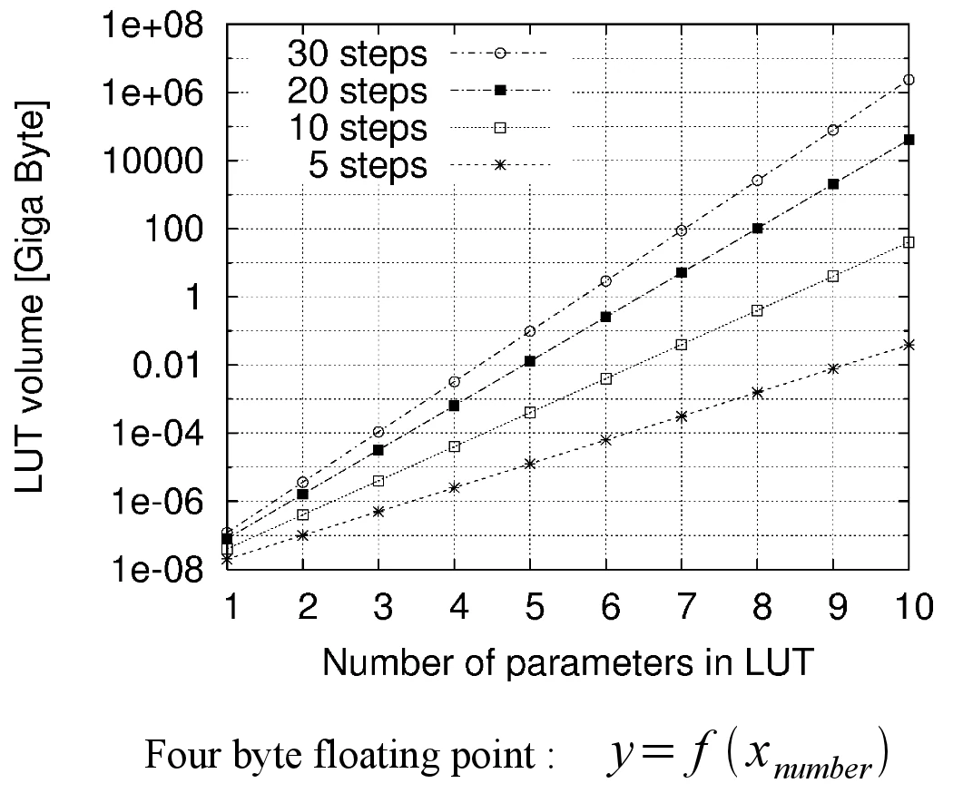
To move beyond this dependence on large LUTs, AMATERASS developed an approach in which a neural network learns the input–output relationship of the radiative transfer model itself.

The neural network does not learn an empirical relationship between satellite observations and ground observations. Instead, it learns the relationship between physical parameters—such as cloud and other particles, absorbing gases, and surface albedo—and the radiative quantities calculated by a detailed radiative transfer model.

Whereas a LUT stores and retrieves discrete precomputed values, a neural network approximates the input–output relationship of the radiative transfer model as a continuous function.

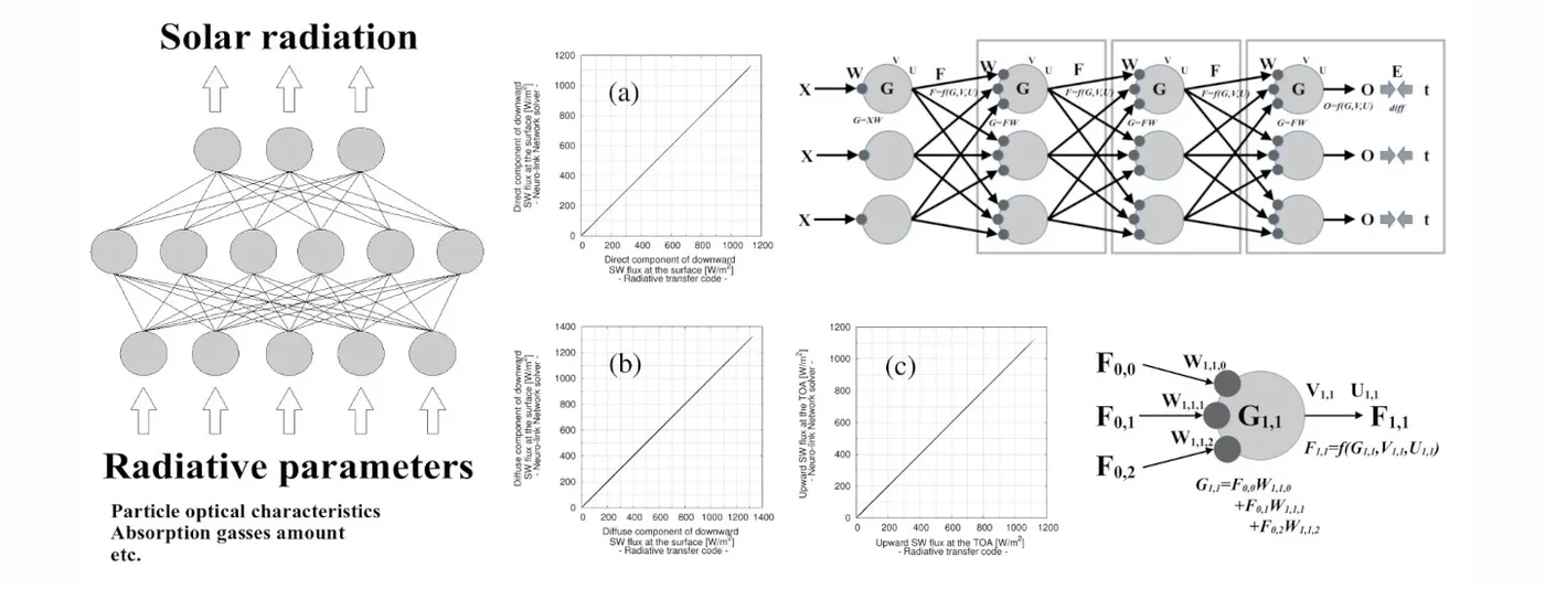
AMATERASS therefore involved not only the use of neural networks, but also the development of learning algorithms that could reproduce complex radiative transfer calculations with high accuracy.

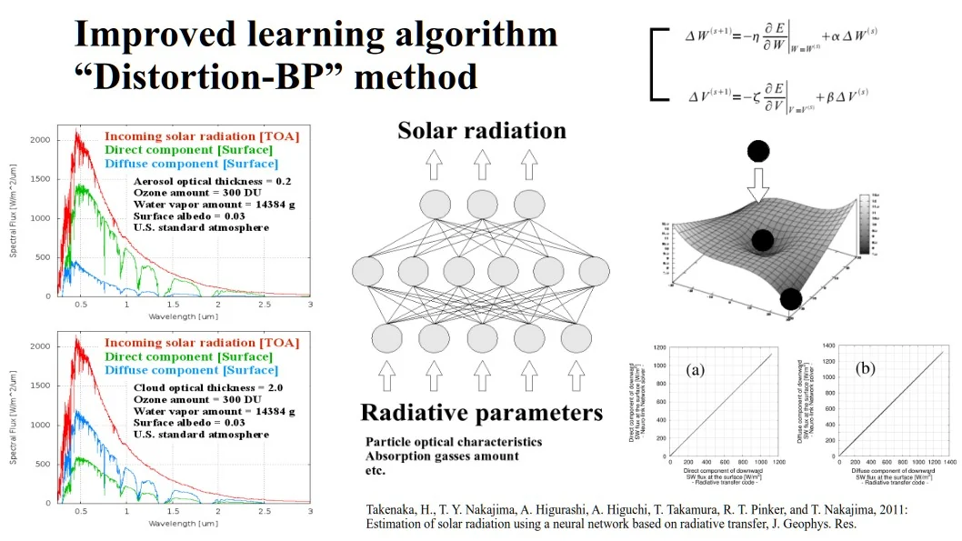
After training, the neural network functions as a radiative-transfer solver, rapidly reproducing the model output instead of rerunning the expensive physical calculation for every pixel. In current terminology, this is close to a surrogate model or emulator. The important point, however, is not the use of a neural network by itself.

This approach brought another major advantage: computational speed. When AMATERASS development began in 2005, detailed solar-radiation analysis using radiative transfer calculations required several seconds per pixel. PCs were still predominantly single-core, and applying the physical model directly to a 3000 × 3000 image—9,000,000 pixels—would require days or longer.

At the time, Himawari performed a full-disk observation once per hour, with a hemispheric scan in between. For quasi-real-time analysis, the computation had to finish before the next observation arrived. Representing the radiative transfer model with a trained neural network removed not only the large-LUT problem but also this computational-speed barrier.

This technology dramatically accelerated radiative transfer calculations.

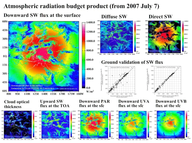
In actual satellite-image processing, an analysis of a 3000 × 3000 image—9 million pixels—that would previously have required days or longer could be completed in a few minutes.

This made it possible to perform detailed physical analysis with a radiative transfer model fast enough to keep pace with the observation cycle of a geostationary meteorological satellite. This was more than a reduction in runtime. It transformed full-image physical analysis, previously impractical because of computational cost, into a continuously operated analysis system.

Moving beyond large LUTs and accelerating the physical calculation were achieved together. That combination made quasi-real-time solar-radiation analysis with AMATERASS possible.

The speedup came from more than simply reducing the number of arithmetic operations with a neural network.

A detailed radiative transfer model accesses many coefficient tables and intermediate variables while performing a complex sequence of calculations. The complete working set is difficult to keep in CPU cache, so data must frequently be transferred to and from main memory. Memory bandwidth was also limited on computers of that era. Even when more CPU cores were used in parallel, the cores had to share the path to memory, and performance per core could decrease.

A trained neural network, by contrast, is extremely compact.

If the network weights and calculation code fit in CPU cache, main memory mainly has to provide input parameters sequentially and receive the output, while most of the computation takes place inside the CPU.

This structure works well with CPU caches and prefetching. As processors moved to dual-core and then multicore designs, the effective processing speed increased further. The large speedup therefore came not only from reducing computation, but also from transforming the problem from one that required extensive data movement into one that could largely execute inside the CPU.

The same principle—performance being governed not only by arithmetic throughput but also by the cost of moving data—is central to modern GPU computing as well.